Introduction
Hello, fellow data enthusiasts! Are you ready to blend the mystical world of finance with the magic of Python? Today, , we’ll dive into implementing SMA Trading Strategy in Python and see it in action with Meta Platforms, Inc. (ticker: META). Ready to blend some finance theory with coding practice? Let’s get cracking!
What is SMA?
The Simple Moving Average (SMA) is as straightforward as its name suggests—it’s the average stock price over a specified number of days, smoothed out to understand underlying trends. It’s like the financial world’s version of ironing out wrinkles on a shirt!
Step 1: Fetch Historical Stock Data for Implementing SMA Trading Strategy in Python
First, we need to pull the historical stock data using yfinance, which helps us fetch financial data directly into Python. This step is like sending out a secret agent to gather intel on stock prices.
Fetching Data
import yfinance as yf

# Fetch historical stock data
def fetch_data(ticker, start, end):
    data = yf.download(ticker, start=start, end=end)
    return data

import yfinance as yf

# Fetch historical stock data
def fetch_data(ticker, start, end):
    data = yf.download(ticker, start=start, end=end)
return dataExplanation: We use yfinance to download the historical data for Meta Platforms, Inc. The fetch_data function takes the stock ticker, start date, and end date, and returns the stock’s historical data. It’s like asking a librarian (Yahoo Finance) to fetch all books (data) on Meta from the library’s archives (the internet).
Step 2: Calculate SMA for Implementing SMA Trading Strategy in Python
Next, we calculate the SMAs. We’ll compute two SMAs—one short (20 days) and one long (50 days). Think of this as smoothing out the ups and downs in the stock price to see the bigger picture.
Calculating SMA
import pandas as pd

# Calculate SMA
def calculate_sma(data, window):
    data[f'SMA_{window}'] = data['Close'].rolling(window=window).mean()
    return data
Explanation: This function adds a new column to our data for each SMA, calculated over the specified window of days. It’s like running a rolling pin over dough to smooth out the lumps, giving us a clearer view of price trends over different periods.
Step 3: Generate Buy/Sell Signals for Implementing SMA Trading Strategy in Python
We now generate the signals. When our short SMA crosses above the long SMA, it’s a buy signal. Conversely, a cross below means sell. This is like getting a green light to buy or a red light to sell.
Generating Signals
# Generate buy/sell signals
def generate_signals(data, short_window, long_window):
    data['Signal'] = 0
    data.loc[data.index[short_window:], 'Signal'] = np.where(
        data.loc[data.index[short_window:], f'SMA_{short_window}'] > data.loc[data.index[short_window:], f'SMA_{long_window}'], 1, 0)
    data['Position'] = data['Signal'].diff()
    return data
Explanation: Here, we initialize the signals to 0 and update them based on our SMA crossover logic. The Position column shows when a new position is opened or closed. Imagine this as a traffic signal at an intersection, directing when you should go (buy) or stop (sell).
Step 4: Evaluate Strategy Performance for Implementing SMA Trading Strategy in Python
Now we calculate the returns from our strategy and compare them to the market returns. This is where the rubber meets the road—we see if our strategy is actually making money!
Evaluating Performance
# Evaluate strategy performance
def evaluate_performance(data):
    data['Market Returns'] = data['Close'].pct_change()
    data['Strategy Returns'] = np.nan  # Initialize strategy returns column with NaN

    entry_price = 0
    for i in range(len(data)):
        if data['Position'].iloc[i] == 1:  # A new position is opened
            entry_price = data['Close'].iloc[i]
        elif data['Position'].iloc[i] == -1 and entry_price != 0:  # An existing position is closed
            exit_price = data['Close'].iloc[i]
            data['Strategy Returns'].iloc[i] = (exit_price - entry_price) / entry_price
            entry_price = 0  # Reset entry price

    data['Strategy Returns'].fillna(0, inplace=True)
    data['Cumulative Market Returns'] = (data['Market Returns'] + 1).cumprod() - 1
    data['Cumulative Strategy Returns'] = (data['Strategy Returns'] + 1).cumprod() - 1
return dataExplanation: This function calculates daily market returns and strategy returns, compounding them to get cumulative returns. It tracks when we open and close positions, calculating returns based on these trades. Think of it as keeping a ledger of all your trades and calculating your profit or loss over time.
Step 5: Plotting the Results for Implementing SMA Trading Strategy in Python
Finally, let’s visualize our data. We’ll plot the stock prices with SMAs, buy/sell signals, cumulative returns, and annual average returns.
Plot Stock Prices with SMAs and Signals
import matplotlib.pyplot as plt

# Plot closing prices and SMAs with signals
def plot_results(data, short_window, long_window):
    plt.figure(figsize=(14, 7))
    plt.plot(data['Close'], label='Close Price', alpha=0.5)
    plt.plot(data[f'SMA_{short_window}'], label=f'SMA_{short_window}', alpha=0.75)
    plt.plot(data[f'SMA_{long_window}'], label=f'SMA_{long_window}', alpha=0.75)

    # Highlight buy and sell signals
    buys = data[data['Position'] == 1]
    sells = data[data['Position'] == -1]
    plt.scatter(buys.index, data['Close'][buys.index], label='Buy Signal', marker='^', color='green', s=100)
    plt.scatter(sells.index, data['Close'][sells.index], label='Sell Signal', marker='v', color='red', s=100)

    plt.title('Stock Price and Moving Averages')
    plt.xlabel('Date')
    plt.ylabel('Price')
    plt.legend()
    plt.show()

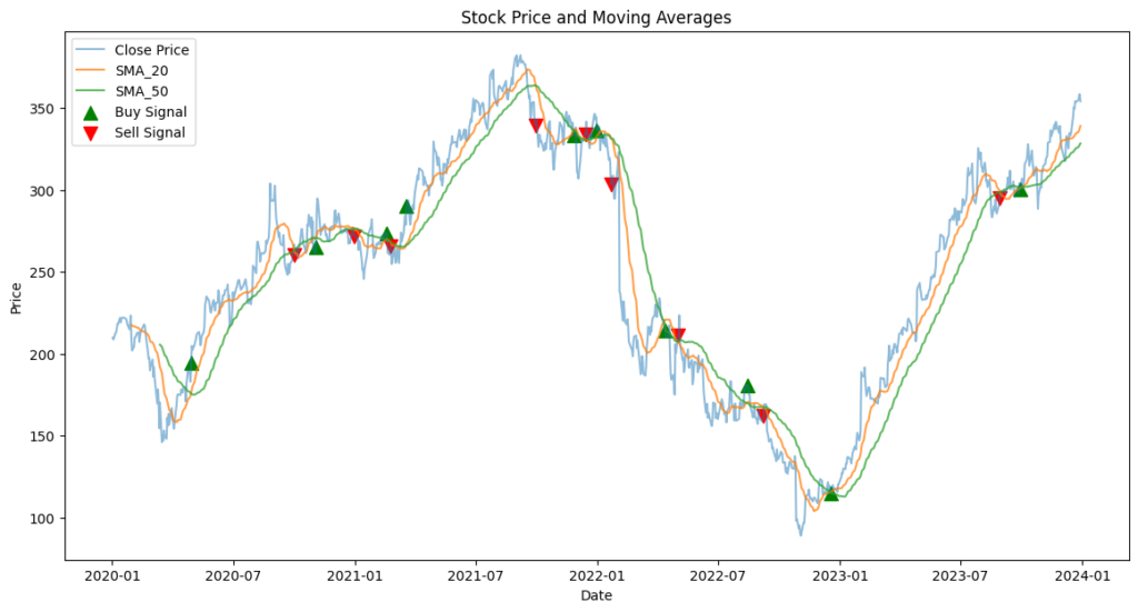
Explanation: This chart shows the price movements with our SMA signals. Green arrows for buying, red arrows for selling. It’s like having a map with all your travel stops marked clearly.
Plot Cumulative Returns
# Plot cumulative returns
def plot_results(data, short_window, long_window):
    # (Include previous plotting code here)

    plt.figure(figsize=(14, 7))
    plt.plot(data['Cumulative Market Returns'] * 100, label='Market Returns (%)')
    plt.plot(data['Cumulative Strategy Returns'] * 100, label='Strategy Returns (%)')
    plt.title('Cumulative Returns Over Time')
    plt.xlabel('Date')
    plt.ylabel('Cumulative Returns (%)')
    plt.legend()
    plt.show()
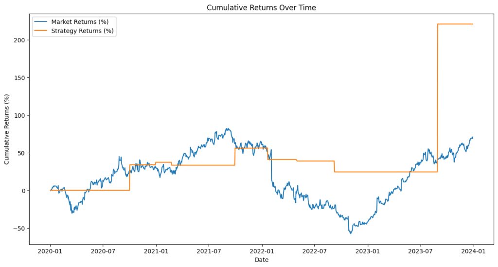
Explanation: This graph compares the strategy’s cumulative returns against the market returns over time. It’s like comparing your road trip progress to see if your route was better than the usual path.
Plot Annual Average Returns
# Annual average returns plot
def plot_results(data, short_window, long_window):
    # (Include previous plotting code here)

    data['Year'] = data.index.year
    annual_market_returns = data.groupby('Year')['Market Returns'].mean() * 252 * 100  # Assuming 252 trading days per year
    annual_strategy_returns = data.groupby('Year')['Strategy Returns'].mean() * 252 * 100

    fig, ax = plt.subplots(figsize=(10, 6))
    index = np.arange(len(annual_market_returns))
    bar_width = 0.35

    rects1 = ax.bar(index, annual_market_returns, bar_width, label='Market Returns (%)')
    rects2 = ax.bar(index + bar_width, annual_strategy_returns, bar_width, label='Strategy Returns (%)')

    ax.set_xlabel('Year')
    ax.set_ylabel('Average Returns (%)')
    ax.set_title('Annual Average Returns')
    ax.set_xticks(index + bar_width / 2)
    ax.set_xticklabels((annual_market_returns.index))
    ax.legend()

    plt.show()
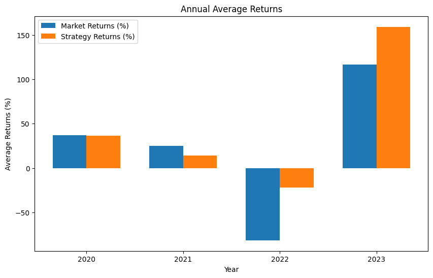
Explanation: This bar chart breaks down the returns year by year, showing when our strategy was a star and when it needed some polish. It’s like an annual report card for our trading strategy.
Commentary on the Results
Stock Price and Moving Averages
In the first graph, we see the stock price of Meta Platforms, Inc. along with the short-term (20 days) and long-term (50 days) SMAs. Green arrows indicate buy signals, and red arrows indicate sell signals. Notice how the buy signals often precede price increases, while sell signals precede price drops. This demonstrates how the SMA strategy helps us catch upward trends and avoid downward spirals.
Cumulative Returns Over Time
The second graph shows the cumulative returns for both the market and our SMA strategy. The market returns, represented by the blue line, show a more volatile journey compared to our SMA strategy. The orange line, representing our strategy, takes a more stair-step approach, reflecting the discrete buy and sell actions. Our SMA strategy significantly outperformed the market, achieving approximately 200% returns compared to the market’s 50%. This highlights the potential of the SMA strategy to yield substantial gains over time while maintaining a more controlled approach.
Annual Average Returns Comparison
The third graph compares the annual average returns for the market and Implementing SMA Trading Strategy in Python. Each pair of bars represents the performance for a specific year.
- 2020: Both the market and our strategy showed modest returns, with the market slightly outperforming the strategy.
- 2021: Our strategy outperformed the market significantly, showcasing its effectiveness in trending markets.
- 2022: A challenging year for both the market and our strategy, with both showing negative returns, but our strategy managed to limit losses better than the market.
- 2023: The strategy outperformed the market by a wide margin, indicating its strong performance during this period.
Overall, this comparison highlights that while the SMA strategy might not always outperform the market, it can provide a more stable and controlled approach to trading, particularly during volatile periods.
Wrapping Up
By Implementing SMA Trading Strategy in Python, we’ve taken a deep dive into both the technical and strategic facets of quantitative trading. Whether you’re a seasoned quant or a curious coder, Python serves as a powerful tool to backtest and visualize trading strategies, making the abstract a little more tangible.
And remember, the market will always have its say, but with tools like Python, we get to whisper back!
Happy Trading!
