Weekly Trading Strategy with Python: Achieving 45.82% Returns with HXT.TO

Understanding the Weekly Trading Strategy with Python

Hey there, fellow investors and coders! Today, we’re exploring an intriguing Weekly trading strategy with Python: buying at the market opening on Mondays and selling at the market close on Fridays. We’ll use Python to analyze ten years of stock data from the Toronto Stock Exchange, specifically the ticker `HXT.TO`, to see how this strategy would have performed. By the end, you’ll see how easy it is to uncover meaningful insights using a bit of code. Let’s get started!

Analyzing HXT.TO: Why This ETF?

Before diving into the analysis, let’s quickly understand what `HXT.TO` is. `HXT.TO` is the ticker symbol for the Horizons S&P/TSX 60 Index ETF on the Toronto Stock Exchange. This ETF aims to replicate the performance of the S&P/TSX 60 Index, which includes 60 of the largest companies listed on the Toronto Stock Exchange. It’s a popular choice among Canadian investors looking for diversified exposure to the Canadian equity market.

Step-by-Step Python Code for the Trading Strategy

First things first, we need to gather our data. We’re using the `yfinance` library to download ten years’ worth of historical data for `HXT.TO`. Here’s the code to get us started:

Step 1: Download Historical Data

import yfinance as yf
import pandas as pd
# Define the ticker and the period for the last 10 years
ticker = 'HXT.TO'
period = '10y'
# Download historical data for the last 10 years
data = yf.download(ticker, period=period)

This script downloads the stock data, giving us the open, high, low, close, volume, and adjusted close prices for each day over the past ten years.This script downloads the stock data, giving us the open, high, low, close, volume, and adjusted close prices for each day over the past ten years.

Step 2: Prepare the Data

Next, we’ll ensure our data is in the right format and assign week and year numbers to each row:

# Ensure that the index is a datetime index
data.index = pd.to_datetime(data.index)
# Assign week and year numbers to each row
data['Week_Number'] = data.index.isocalendar().week
data['Year'] = data.index.year

By converting the index to a datetime index and adding week and year columns, we set the stage for more detailed analysis.

Step 3: Filter for Weekly Data

We want to focus on our strategy: buying on Mondays and selling on Fridays. So, we’ll filter out the data to only include Mondays and Fridays:

# Filter out the data to only include Mondays and Fridays
mondays = data[data.index.weekday == 0] # 0 is Monday
fridays = data[data.index.weekday == 4] # 4 is Friday

This snippet helps us capture the opening price on the first day of the week (Monday) and the closing price on the last day of the week (Friday).

Step 4: Calculate Weekly Returns

Now, let’s calculate the weekly returns by comparing the Monday open to the Friday close:

# Get the opening price of the first Monday and closing price of the last Friday of each week
weekly_opens = mondays.groupby(['Week_Number', 'Year'])['Open'].first()
weekly_closes = fridays.groupby(['Week_Number', 'Year'])['Close'].last()
# Combine weekly opens and closes into a single DataFrame
weekly_data = pd.merge(weekly_opens.reset_index(), weekly_closes.reset_index(), on=['Week_Number', 'Year'], how='inner')
# Calculate weekly returns
weekly_data['Weekly_Return'] = (weekly_data['Close'] - weekly_data['Open']) / weekly_data['Open']

By grouping the data by week and year, we get the first open and last close for each week. The weekly return is then calculated as the percentage change from Monday’s open to Friday’s close.

Step 5: Calculate Annual and Cumulative Returns

To see the bigger picture, we’ll calculate the annual returns and the cumulative return over the entire period:

# Calculate the annual returns
annual_returns = weekly_data.groupby('Year')['Weekly_Return'].sum()
# Calculate cumulative returns
cumulative_returns = (1 + weekly_data['Weekly_Return']).cumprod() - 1
# Display the results
if not weekly_data.empty:
 print("Annual Returns by Year:")
 print((annual_returns * 100).round(2).astype(str) + '%') # Convert to percentage and format as string
 print("\nCumulative Return:")
 print(f"{cumulative_returns.iloc[-1] * 100:.2f}%")
else:
 print("No matching data for Mondays or Fridays within the provided timeframe.")

This part sums up the weekly returns for each year to give us annual returns. The cumulative return is calculated by compounding the weekly returns.

Results: Cumulative Returns and Insights

Here are the results of our analysis:

Annual Returns by Year:

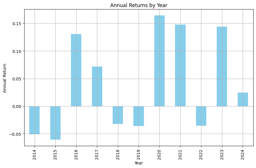
Weekly trading strategy with Python for HXT.TO showing an annual returns over the last 10 years

Cumulative Return:

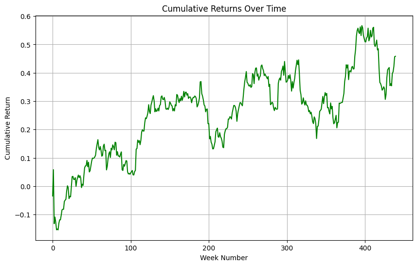
• 45.82%

These numbers tell us that while there have been ups and downs, the stock has grown significantly over the past decade, with a cumulative return of 45.82%.

Conclusion: Applying the Weekly Trading Strategy

This weekly trading strategy with Python of buying `HXT.TO` at the opening price on Mondays and selling it at the closing price on Fridays showed a considerable cumulative return over ten years. While the strategy had its ups and downs, it highlights an interesting approach to trading that you can explore further. Give it a try with your favorite stock and see what insights you can uncover!

Happy investing and coding!