Introduction
Hey there, finance wizards and data enthusiasts! Ever wondered how we can predict the future of our economy using a bit of Python magic and some machine learning? Today, we’re going to dive into the world of economic forecasting by predicting GDP with Gradient Boosting. We’ll make it fun, engaging, and packed with insights. So, grab your favorite snack, sit back, and let’s get our hands dirty with some data!
What is GDP?
Gross Domestic Product (GDP) is like the report card for a country’s economy. It’s the total monetary value of all goods and services produced within a country’s borders over a specific period. When GDP is on the rise, it means the economy is doing well and people are likely spending and investing more. When it’s down, well, let’s just say it’s not the best news for anyone. So, predicting GDP can give us a sneak peek into the economic future, helping businesses, policymakers, and investors make informed decisions.
What is the FRED API?
Imagine having a treasure chest filled with all sorts of economic data—GDP, unemployment rates, inflation, you name it. That’s the FRED API (Federal Reserve Economic Data). It’s a web service provided by the Federal Reserve Bank of St. Louis that lets you fetch a vast array of economic data directly into your Python scripts. Think of it as your secret weapon for economic analysis, providing up-to-date data at your fingertips.
What is Gradient Boosting?
Now, let’s talk about Gradient Boosting. Picture yourself building a Lego tower. Each block represents a small, simple model (we call them “weak learners”). Gradient Boosting stacks these blocks one by one, each time correcting the errors made by the previous block, until we have a mighty tower (a strong predictive model). It’s a powerful machine learning technique used for regression and classification tasks. In our case, we’ll use be predicting GDP with Gradient Boosting on various economic indicators.
Data Preparation
First things first, we need some data. We’ll use the FRED API to fetch GDP and other economic indicators. Here’s how we do it:
Fetching the Data
We need several key economic indicators to make accurate predictions. Here are the ones we selected and why:
- Unemployment Rate (UNRATE): High unemployment can signal a struggling economy, while low unemployment indicates economic growth.
- Inflation (CPIAUCSL): Inflation rates can impact purchasing power and economic stability.
- Interest Rate (DFF): The federal funds rate affects borrowing costs and economic activity.
- Consumer Sentiment (UMCSENT): Reflects consumer confidence, which influences spending and investment.
- Industrial Production (INDPRO): Measures the output of the industrial sector, a major component of the economy.
Let’s fetch the data using the FRED API:
import pandas as pd
from fredapi import Fred

# Initialize FRED API with your API key
fred = Fred(api_key='6a7adb693d4cfda849e37ad329d7076c')

# Download GDP data from FRED
gdp = fred.get_series('GDP')

# Download other economic indicators as features
unemployment = fred.get_series('UNRATE')
inflation = fred.get_series('CPIAUCSL')
interest_rate = fred.get_series('DFF')
consumer_sentiment = fred.get_series('UMCSENT')
industrial_production = fred.get_series('INDPRO')
Combining and Cleaning the Data
Now, let’s combine all this data into a single DataFrame and clean it up:
# Combine the data into a single DataFrame
data = pd.concat([gdp, unemployment, inflation, interest_rate, consumer_sentiment, industrial_production], axis=1).dropna()
data.columns = ['GDP', 'Unemployment Rate', 'Inflation', 'Interest Rate', 'Consumer Sentiment', 'Industrial Production']

# Shift the target column (GDP) one row up to predict the next value
data['GDP'] = data['GDP'].shift(-1)
data = data.dropna()
Building the Gradient Boosting Model
With our data ready, it’s time to build and train our model to start predicting GDP with Gradient Boosting.
Splitting the Data
First, we’ll split our data into training and testing sets:
from sklearn.model_selection import train_test_split

# Prepare features and target
features = ['Unemployment Rate', 'Inflation', 'Interest Rate', 'Consumer Sentiment', 'Industrial Production']
target = 'GDP'
X = data[features]
y = data[target]

# Split data into training and testing sets
X_train, X_test, y_train, y_test = train_test_split(X, y, test_size=0.2, random_state=42)
Training the Model
Next, we’ll initialize and train our Gradient Boosting model:
from sklearn.ensemble import GradientBoostingRegressor

# Initialize and train the Gradient Boosting model
gbr = GradientBoostingRegressor(n_estimators=100, learning_rate=0.1, max_depth=3, random_state=42)
gbr.fit(X_train, y_train)
Model Evaluation
Let’s see how our model performed. We’ll evaluate it using Mean Squared Error (MSE) and R-squared (R²) metrics.
Making Predictions
First, we’ll make predictions on our test set:
# Make predictions
y_pred = gbr.predict(X_test)
Evaluating the Model
Now, let’s evaluate the model’s performance:
from sklearn.metrics import mean_squared_error, r2_score

# Evaluate the model
mse = mean_squared_error(y_test, y_pred)
r2 = r2_score(y_test, y_pred)

print(f'Mean Squared Error: {mse}')
print(f'R-squared: {r2}')
What are Mean Squared Error and R-squared?
Mean Squared Error (MSE) measures the average squared difference between the predicted and actual values. It’s a way to quantify how well the model’s predictions match the actual data. The lower the MSE, the better the model’s performance.
R-squared (R²), on the other hand, is a statistical measure that represents the proportion of the variance for the dependent variable (GDP, in this case) that’s explained by the independent variables in the model. An R² value closer to 1 indicates that the model explains a large portion of the variance, while an R² value closer to 0 indicates that the model doesn’t explain much of the variance.
Visualization
Visualizing our results helps us understand the model’s performance better. We will use two types of graphs to analyze the performance of our model:
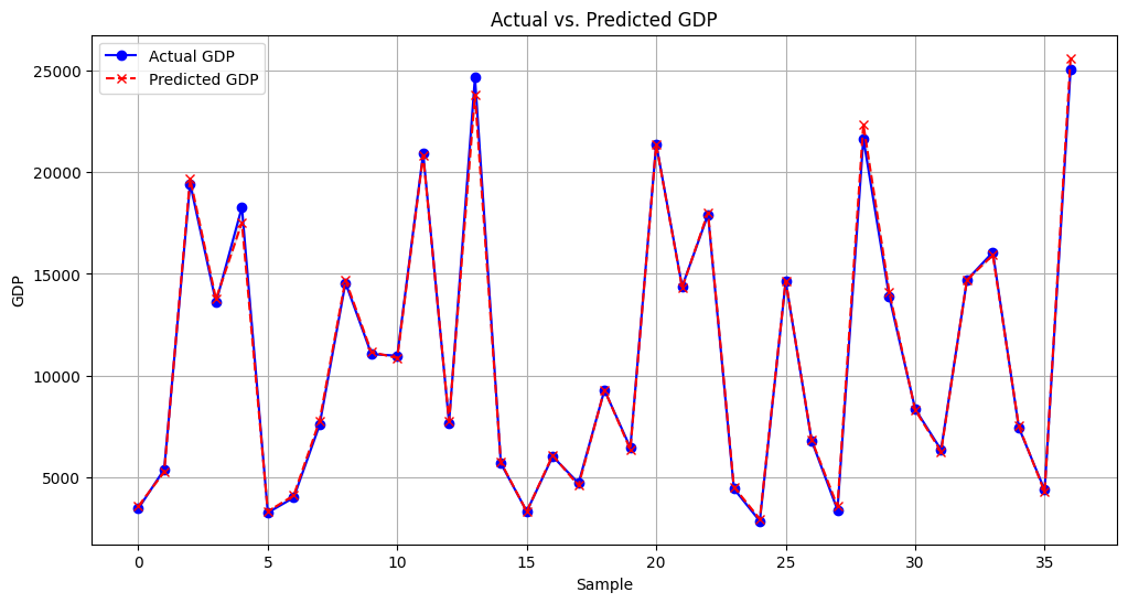
- Actual vs. Predicted GDP Plot: This graph will show the comparison between the actual GDP values and the GDP values predicted by our model. It helps us visually assess how closely predicting GDP with Gradient Boosting match the real data.
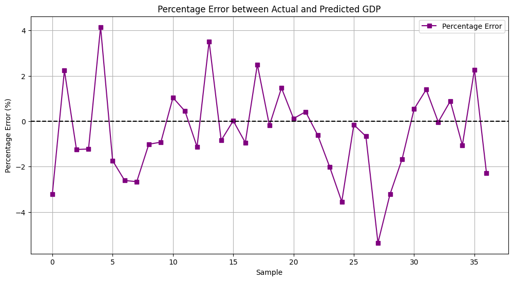
- Percentage Error Plot: This graph will display the percentage error between the actual and predicted GDP values. It helps us understand the accuracy of our predictions in relative terms.
Actual vs. Predicted GDP
Here’s a plot of the actual vs. predicted GDP:
import matplotlib.pyplot as plt

plt.figure(figsize=(12, 6))
plt.plot(y_test.values, label='Actual GDP', color='blue', marker='o')
plt.plot(y_pred, label='Predicted GDP', color='red', linestyle='dashed', marker='x')
plt.fill_between(range(len(y_test)), y_test, y_pred, color='gray', alpha=0.2)
plt.xlabel('Sample')
plt.ylabel('GDP')
plt.title('Actual vs. Predicted GDP')
plt.legend()
plt.grid(True)
plt.show()

Percentage Error
And here’s a plot of the percentage error between actual and predicted GDP:
# Plot the percentage error between actual and predicted GDP
percentage_error = (y_test.values - y_pred) / y_test.values * 100
plt.figure(figsize=(12, 6))
plt.plot(percentage_error, label='Percentage Error', color='purple', marker='s')
plt.axhline(y=0, color='black', linestyle='--')
plt.xlabel('Sample')
plt.ylabel('Percentage Error (%)')
plt.title('Percentage Error between Actual and Predicted GDP')
plt.legend()
plt.grid(True)
plt.show()
Predicting GDP with Gradient Boosting : Interpretation and Insights
Now, let’s interpret our results. The actual vs. predicted GDP plot shows how closely our model’s predictions match the real GDP values. Predicting GDP with Gradient Boosting The percentage error plot helps us understand the prediction accuracy in relative terms.
Looking at the percentage error graph, we can see that the maximum absolute percentage error is around 4%. This indicates that our model rarely deviates significantly from the actual values, which is excellent for economic forecasting. The average absolute error percentage of predicting GDP with Gradient Boosting is around 2%, showing that on average, our predictions are very close to the real GDP values.
This low error margin suggests that Predicting GDP with a Gradient Boosting model is highly effective in capturing the underlying patterns in the data. Such accuracy is crucial for making reliable economic predictions, which can help policymakers, investors, and businesses make informed decisions.
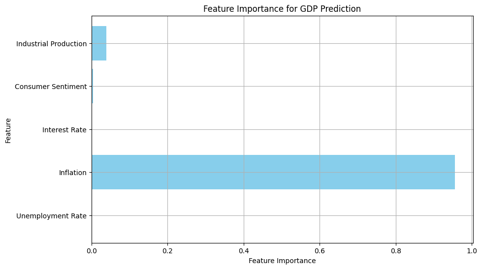
Additionally, the feature importance plot reveals that certain indicators, such as inflation and industrial production, play significant roles in predicting GDP. Understanding these relationships can provide deeper insights into the economic factors driving GDP changes.
In conclusion, the model demonstrates great performance with minimal prediction errors, making it a valuable tool for economic forecasting. The insights gained from feature importance further enhance our understanding of the key drivers of GDP.
What is Feature Importance?
Feature Importance is a technique used to understand the contribution of each feature to the prediction made by a machine learning model. In simpler terms, it helps us identify which variables (features) are most influential in predicting the target variable (in our case, GDP). By analyzing feature importance, we can gain insights into which economic indicators have the most significant impact on GDP predictions.
Here’s how we can visualize feature importance:
# Plot feature importance
plt.figure(figsize=(10, 6))
feature_importance = gbr.feature_importances_
plt.barh(features, feature_importance, color='skyblue')
plt.xlabel('Feature Importance')
plt.ylabel('Feature')
plt.title('Feature Importance for GDP Prediction')
plt.grid(True)
plt.show()
Conclusion
We’ve successfully built a Gradient Boosting model to predict GDP using macroeconomic indicators. The model shows promising results, and by analyzing feature importance, we can gain valuable insights into the factors driving GDP.
In future articles, we’ll explore more advanced techniques and improvements to refine our predictions. Stay tuned, and happy forecasting!
