
Algorithmic trading is a game-changer in quantitative finance. It leverages financial modeling and quantitative analysis to create robust strategies that can be backtested and optimized. In this tutorial, we’ll build a simple algorithmic trading strategy using Python, focusing on the Relative Strength Index (RSI) and Moving Average Crossover. Plus, we’ll optimize the RSI period to see how it impacts performance.
Introduction to Quantitative Finance and Algorithmic Trading
Algorithmic trading uses computer algorithms to execute trading strategies at high speed and frequency. These strategies can be based on various factors, such as price, volume, and time. The advantages include improved order execution, the ability to backtest strategies, and reduced emotional bias.
Understanding RSI and Moving Averages in Quantitative Finance
Relative Strength Index (RSI): The RSI is a momentum oscillator that measures the speed and change of price movements. It ranges from 0 to 100 and helps identify overbought or oversold conditions.
Moving Averages: Moving averages smooth out price data to identify trends. The Simple Moving Average (SMA) is the average price over a specific period, while the Exponential Moving Average (EMA) gives more weight to recent prices.
Crossovers: A crossover occurs when a shorter moving average crosses above or below a longer moving average, signaling a potential trend change.
Setting Up Your Python Environment
To get started, install the necessary Python libraries. You can do this using pip:
pip install pandas numpy matplotlib yfinance ta-libBuilding the Trading Strategy
Step 1: Import Libraries
First, import the necessary libraries:
import pandas as pd
import numpy as np
import yfinance as yf
import matplotlib.pyplot as plt
import talib
Step 2: Download Historical Data
Next, download historical data for SPY from Yahoo Finance:
data = yf.download('SPY', start='2020-01-01', end='2023-01-01')
data['Adj Close'].plot(title='SPY Adjusted Close Price', figsize=(12, 6))
plt.show()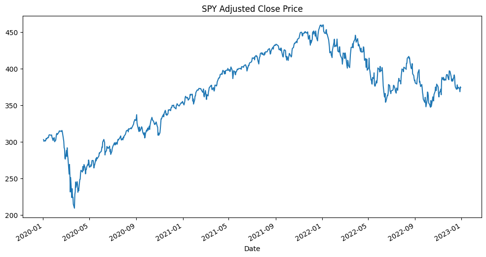
Step 3: Calculate RSI in Quantitative Finance
Calculate the RSI using the quantitative finance talib library:
data['RSI'] = talib.RSI(data['Adj Close'], timeperiod=14)Step 4: Calculate Moving Averages in Quantitative Finance
Calculate the 50-day and 200-day Simple Moving Averages (SMA):
data['SMA50'] = data['Adj Close'].rolling(window=50).mean()
data['SMA200'] = data['Adj Close'].rolling(window=200).mean()
Step 5: Define the Trading Strategy
Define the trading strategy using RSI and Moving Average Crossover:
data['Buy_Signal'] = (data['RSI'] < 30) & (data['SMA50'] > data['SMA200'])
data['Sell_Signal'] = (data['RSI'] > 70) & (data['SMA50'] < data['SMA200'])
Step 6: Plot the Strategy Signals
Finally, plot the strategy signals on the price chart:
plt.figure(figsize=(12, 6))
plt.plot(data['Adj Close'], label='SPY')
plt.plot(data['SMA50'], label='50-Day SMA')
plt.plot(data['SMA200'], label='200-Day SMA')

# Plot Buy and Sell signals
buy_signals = data[data['Buy_Signal']]
sell_signals = data[data['Sell_Signal']]

plt.scatter(buy_signals.index, buy_signals['Adj Close'], marker='^', color='g', label='Buy Signal', alpha=1)
plt.scatter(sell_signals.index, sell_signals['Adj Close'], marker='v', color='r', label='Sell Signal', alpha=1)

plt.title('SPY Trading Strategy Signals')
plt.legend()
plt.show()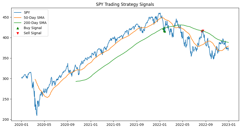
Backtesting the Strategy
Step 1: Initialize Portfolio
Initialize the portfolio with initial cash:
initial_cash = 100000
data['Position'] = 0
data.loc[data['Buy_Signal'], 'Position'] = 1
data.loc[data['Sell_Signal'], 'Position'] = -1
data['Position'] = data['Position'].replace(to_replace=0, method='ffill')
data['Daily_Return'] = data['Adj Close'].pct_change()
data['Strategy_Return'] = data['Daily_Return'] * data['Position'].shift()
Step 2: Calculate Cumulative Returns
Calculate the cumulative returns for the strategy and the market:
data['Cumulative_Strategy_Return'] = (1 + data['Strategy_Return']).cumprod() * initial_cash
data['Cumulative_Market_Return'] = (1 + data['Daily_Return']).cumprod() * initial_cash
Step 3: Plot the Results
Plot the cumulative returns to compare the strategy performance against the market:
plt.figure(figsize=(12, 6))
plt.plot(data['Cumulative_Strategy_Return'], label='Strategy Return')
plt.plot(data['Cumulative_Market_Return'], label='Market Return')
plt.title('Cumulative Returns')
plt.legend()
plt.show()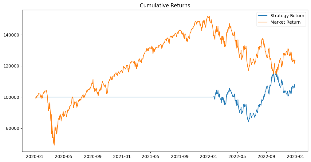
Optimizing the Strategy
Step 1: Optimize RSI Period
Optimize the RSI period to find the best performance:
best_period = 14
best_performance = 0

for period in range(10, 21):
    data['RSI'] = talib.RSI(data['Adj Close'], timeperiod=period)
    data['Buy_Signal'] = (data['RSI'] < 30) & (data['SMA50'] > data['SMA200'])
    data['Sell_Signal'] = (data['RSI'] > 70) & (data['SMA50'] < data['SMA200'])
    data['Position'] = 0
    data.loc[data['Buy_Signal'], 'Position'] = 1
    data.loc[data['Sell_Signal'], 'Position'] = -1
    data['Position'] = data['Position'].replace(to_replace=0, method='ffill')
    data['Strategy_Return'] = data['Daily_Return'] * data['Position'].shift()
    cumulative_return = (1 + data['Strategy_Return']).cumprod()[-1]

    if cumulative_return > best_performance:
        best_performance = cumulative_return
        best_period = period

print(f"Best RSI period: {best_period}")
Best RSI period: 10
Running the Optimized Strategy
Step 1: Update RSI with Best Period
Update the RSI calculation with the best period found during optimization:
data['RSI'] = talib.RSI(data['Adj Close'], timeperiod=best_period)
data['Buy_Signal'] = (data['RSI'] < 30) & (data['SMA50'] > data['SMA200'])
data['Sell_Signal'] = (data['RSI'] > 70) & (data['SMA50'] < data['SMA200'])
data['Position'] = 0
data.loc[data['Buy_Signal'], 'Position'] = 1
data.loc[data['Sell_Signal'], 'Position'] = -1
data['Position'] = data['Position'].replace(to_replace=0, method='ffill')
data['Strategy_Return'] = data['Daily_Return'] * data['Position'].shift()
Step 2: Plot the Strategy Signals
Plot the strategy signals on the price chart:
# Plot the strategy signals after optimization
plt.figure(figsize=(12, 6))
plt.plot(data['Adj Close'], label='SPY')
plt.plot(data['SMA50'], label='50-Day SMA')
plt.plot(data['SMA200'], label='200-Day SMA')

# Plot Buy and Sell signals
buy_signals = data[data['Buy_Signal']]
sell_signals = data[data['Sell_Signal']]

plt.scatter(buy_signals.index, buy_signals['Adj Close'], marker='^', color='g', label='Buy Signal', alpha=1)
plt.scatter(sell_signals.index, sell_signals['Adj Close'], marker='v', color='r', label='Sell Signal', alpha=1)

plt.title('SPY Trading Strategy Signals After Optimization')
plt.legend()
plt.show()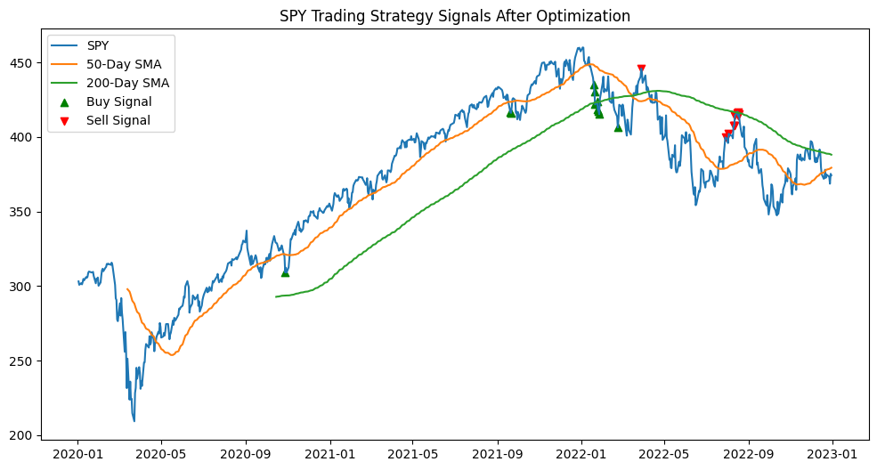
Step 3: Calculate and Plot Optimized Returns
Calculate and plot the cumulative returns for the optimized strategy:
data['Cumulative_Strategy_Return'] = (1 + data['Strategy_Return']).cumprod() * initial_cash
data['Cumulative_Market_Return'] = (1 + data['Daily_Return']).cumprod() * initial_cash

plt.figure(figsize=(12, 6))
plt.plot(data['Cumulative_Strategy_Return'], label='Optimized Strategy Return')
plt.plot(data['Cumulative_Market_Return'], label='Market Return')
plt.title('Cumulative Returns After Optimization')
plt.legend()
plt.show()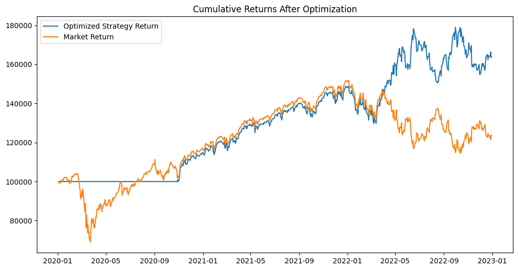
Analysis and Conclusion
Analysis Before Optimization
Without optimization, the strategy generates only a few buy and sell signals. As shown in the cumulative returns chart, the strategy underperforms the market. Specifically, our initial investment of $100,000 ends the period with approximately $109,000, while the market (S&P 500) rises to about $121,000. The strategy reaches its lowest value of $83,500 in June 2022. This underperformance indicates that the initial parameters for the RSI period and moving averages may not be optimal.
Analysis After Optimization
After optimizing the RSI period, we find that the best period is 10. This generates more buy and sell signals, significantly improving performance. Our optimized strategy portfolio value rises to approximately $163,000, outperforming the market which stands at $119,832. The optimized strategy not only recovers from the initial underperformance but also provides a substantial gain.
Here’s a closer look at the performance improvements:
- Number of Signals: The optimized strategy generates more frequent buy and sell signals, providing more opportunities for profit.
- Performance Metrics: Our strategy portfolio value increases to $163,000 from an initial investment of $100,000, while the market value is $119,832. This represents a 63% return compared to the market’s 19.83% return.
- Market Conditions: The optimized strategy performs well in both trending and sideways markets, thanks to the improved timing of buy and sell signals.
Conclusion
In this tutorial, we built and optimized a simple Quantitative Finance algorithmic trading strategy using Python. By combining RSI and Moving Average Crossover, we created a strategy that identifies potential buy and sell signals. We also optimized the RSI period to improve performance. The results show that optimization can significantly enhance strategy performance, turning an underperforming strategy into a profitable one.
Experiment with the code, optimize parameters, and adapt the strategy to suit your trading needs. Remember, the key to successful algorithmic trading is continuous learning and adaptation. Happy trading!